
 Sample Submission Guidelines
Pan-genome Analysis: Statistical Profiling and Visualization of Four Gene Categories
This article presents a comprehensive framework for pan-genome analysis, emphasizing the classification of genes into core, softcore, dispensable, and private categories based on presence/absence frequency across genomes. Using the PSVCP pipeline and OrthoFinder, we construct a linear pan-genome, detect structural variants, and identify orthologous gene families. A statistical workflow is implemented to assign gene categories and quantify their distribution. Visualization techniques-including pie charts, histograms, bar charts, and heatmaps-highlight genomic diversity and population structure. This approach enables deeper insights into genome evolution, functional differentiation, and adaptive traits, supporting applications in plant breeding, microbial studies, and disease genomics.
1. Pan-genome Overview
What is a Pan-genome?
The pan-genome represents the full complement of genes in a defined group of organisms-encompassing both shared and variable genomic content across individuals or species. Unlike the traditional approach of analyzing a single reference genome, the pan-genome embraces intra-species genomic diversity, enabling more comprehensive insights into structural variation, gene presence/absence variation (PAV), and evolutionary dynamics.
Originally proposed in bacterial genomics, the pan-genome concept has since evolved into a central paradigm in plant breeding, microbial adaptation, and cancer genomics.
Historical Context and Relevance
The term "pan-genome" was first coined in 2005 by Tettelin et al. during comparative analysis of multiple Streptococcus agalactiae strains. Their work illuminated the limitations of reference-only analysis, advocating for a more inclusive model of genome content. Since then, the concept has revolutionized:
- Crop genomics: Revealing missing genes from reference assemblies
- Microbial studies: Mapping gene acquisition, horizontal gene transfer
- Oncology: Understanding tumor heterogeneity and mutation hotspots
Why Classify Genes into Four Categories?
Pan-genome analysis reveals that not all genes are equally distributed across individuals. Stratifying genes into core, softcore, dispensable, and private categories provides a quantitative framework for:
- Prioritizing functional genomic studies
- Linking genotype to phenotype
- Disentangling evolutionary selection from stochastic variation
Services you may interested in
Learn More
2. Classification of Gene Categories in Pan-genome Analysis
2.1 Definitions and Criteria
In pan-genomic studies, gene families are typically categorized based on their presence across samples. Core genes are universally conserved and appear in all individuals of the population, suggesting their essential biological roles. Softcore genes, though not strictly universal, are found in more than 90% of individuals and may reflect strong evolutionary conservation with minor population-specific variability. Dispensable genes are present in a subset of individuals, typically more than one but less than 90%, and often correspond to genes involved in environmental response, immunity, or stress adaptation. Finally, private genes are exclusive to a single genome within the dataset, indicating possible recent insertions, structural variants, or annotation artifacts. This classification serves as the foundation for downstream statistical and functional analysis.
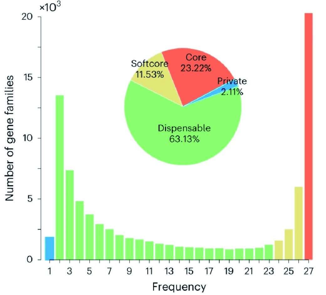 Figur1 . Composition of the syntenic pan-genome.(Li, X. et al, 2024)
2.2 Biological Implications
Core genes often encode essential functions related to cellular maintenance, development, and reproduction.
Softcore genes may reflect environment-specific adaptations or subpopulation-specific conservation.
Dispensable genes drive phenotypic diversity and are often enriched in stress response, immunity, and secondary metabolism.
Private genes might represent recent insertions, horizontal transfer events, or artifacts of assembly or annotation.
3. Pan-genome Construction and SV Calling with PSVCP
The psvcp_v1.01 pipeline facilitates the construction of a linear pan-genome and identifies population-scale structural variations (SVs) from short-read data.
Key Steps:
Input: Assembled genome FASTAs, annotations (GFF), and population sequencing data
Step 1: Download the psvcp_v1.01 pipeline
git clone https://github.com/wjian8/psvcp_v1.01.git
Step 2: Merge reference genomes via Genome_construct_Pangenome.py
#constructing a linear pan-genome by two genome
bash $path_of_the_pipeline/Refgenome_update_by_quest.sh ref.fa query.fa > job.sh && bash job.sh
#constructing pan-genome by several (more than 2) genome
python3 $path_of_the_pipeline/1Genome_construct_Pangenome.py genome_example_dir genome_list
Step 3: Map reads to pan-genome using Map_fq_to_Pan.py
python3 $path_of_the_pipeline/2Map_fq_to_Pan.py -t 4 -fqd fq_dir -r ReferenceFile -br bam_dir
Step 4: Call SVs (PAVs, inversions, translocations) and generate genotype matrix with Call_sv_to_genotype.py
python3 $path_of_the_pipeline/3Call_sv_to_genotype.py -br bam_dir -o hmp_prefix
the ouput file is the prefix of a genotype file which is hapmap format.
4. Pan-genome Ortholog Detection with OrthoFinder
To reliably track gene families across individuals, OrthoFinder is employed to detect orthogroups across multiple genomes, thereby grouping genes that evolved from a common ancestor. It also resolves gene duplications and losses, offering insights into gene family evolution and lineage-specific expansions or contractions. Additionally, OrthoFinder identifies syntenic blocks, which are conserved gene orders across genomes, facilitating collinearity analysis and enhancing the accuracy of orthologous gene assignment in pan-genome studies.
Step 1: Install OrthoFinder
conda install orthofinder -c bioconda
Step 2: Running OrthoFinder
"OrthoFinder/ExampleData" with the directory containing your input fasta files, with one file per species.
OrthoFinder/orthofinder -f OrthoFinder/ExampleData
A typical OrthoFinder run generates a comprehensive collection of output files, including information on orthogroups, orthologous relationships, gene trees, resolved gene trees, the rooted species tree, gene duplication events, and comparative genomic statistics across the analyzed species. All results are organized within a well-structured and user-friendly directory layout for easy navigation and interpretation.
5. Pan-genome Statistical Profiling of Gene Categories
5.1 Input Data Requirements
The analysis requires a binary orthogroup presence/absence matrix in which each row represents an orthogroup (gene family) and each column represents a sample (genome). Entries indicate whether a given orthogroup is present (1) or absent (0) in each sample. Optionally, metadata such as sample origin, phenotype, or ecological context can be integrated for downstream stratified analyses.
5.2 Workflow for Gene Category Assignment
To stratify genes into core, softcore, dispensable, and private categories, the following steps are implemented:
Step 1: Calculate Frequency of Gene Presence
The frequency of each orthogroup across samples is calculated as the proportion of genomes in which the gene is present.
library(tidyverse)

# Load orthogroup gene count matrix and unassigned gene table
df <- read.csv('Orthogroups.GeneCount.tsv', sep = '\t', row.names = 1)
df_uniq <- read.csv('Orthogroups_UnassignedGenes.tsv', sep = '\t', row.names = 1)

# Remove the last column if it contains summary statistics
df <- df[, 1:(ncol(df) - 1)]

# Convert unassigned gene table to binary format
df_uniq[df_uniq != ''] <- 1
df_uniq[df_uniq == ''] <- 0

# Merge assigned and unassigned gene tables
df_combined <- rbind(df, df_uniq)
df_combined[is.na(df_combined)] <- 0 # Fill NA with 0
To illustrate the workflow, we simulate a random presence/absence matrix.
set.seed(123)
n_genes <- 1000
n_samples <- 27

gene_categories <- sample(c("Core", "Softcore", "Dispensable", "Private"),
  n_genes,
  replace = TRUE,
  prob = c(0.20, 0.15, 0.55, 0.1))

binary_matrix <- sapply(gene_categories, function(cat) {
 switch(cat,
 "Core" = rep(1, n_samples),
 "Softcore"= rbinom(n_samples, 1, 0.95),
 "Private" = rbinom(n_samples, 1, 0.05),
 "Dispensable" = rbinom(n_samples, 1, 0.5)
 )
}) %>% t()

colnames(binary_matrix) <- paste0("Genome_", 1:n_samples)
rownames(binary_matrix) <- paste0("Gene_", 1:n_genes)
df_combined <- as.data.frame(binary_matrix)
Step 2: Assign Gene Categories Based on Frequency Thresholds
Each gene is classified into one of four categories:
 # Calculate presence frequency for each gene
df_summary <- data.frame(
 gene = rownames(df_combined),
 frequency = apply(df_combined, 1, function(x) sum(x != 0) / ncol(df_combined)),
 stringsAsFactors = FALSE
)
df_summary<-df_summary[!df_summary$frequency==0,]
# Assign gene category based on frequency
df_summary$Category <- with(df_summary, case_when(
 frequency == 1 ~ "Core",
 frequency >= 0.9 ~ "Softcore",
 frequency == 1 / ncol(df_combined) ~ "Private",
 TRUE ~ "Dispensable"
))
Step 3: Generate Summary Statistics
Once classified, a statistical summary is produced to quantify the distribution of gene categories:
 # Count number of genes in each category
table(df_summary$Category)

# Calculate category proportions
prop.table(table(df_summary$Category))
This includes the total count and proportion of genes in each category.
6. Pan-genome Visualization of Gene Category Distribution
To facilitate intuitive interpretation of pan-genomic structure and gene category dynamics, several visualization strategies are employed:
6.1 Pie Charts
Purpose: Visualize the proportion of genes in each category.
ggplot(df_summary, aes(x = "", fill = Category)) +
 geom_bar(width = 1, color = "white") +
 coord_polar("y") +
 theme_void() +
 scale_fill_manual(values = c("#F8766D", "#7CAE00", "#00BFC4", "#C77CFF")) +
 geom_text(aes(label = paste0(round(..count../sum(..count..)*100, 2), "%")),
 stat = "count",
 position = position_stack(vjust = 0.5),
 color = "black", size = 4)
This provides an immediate overview of the genome-wide gene composition.
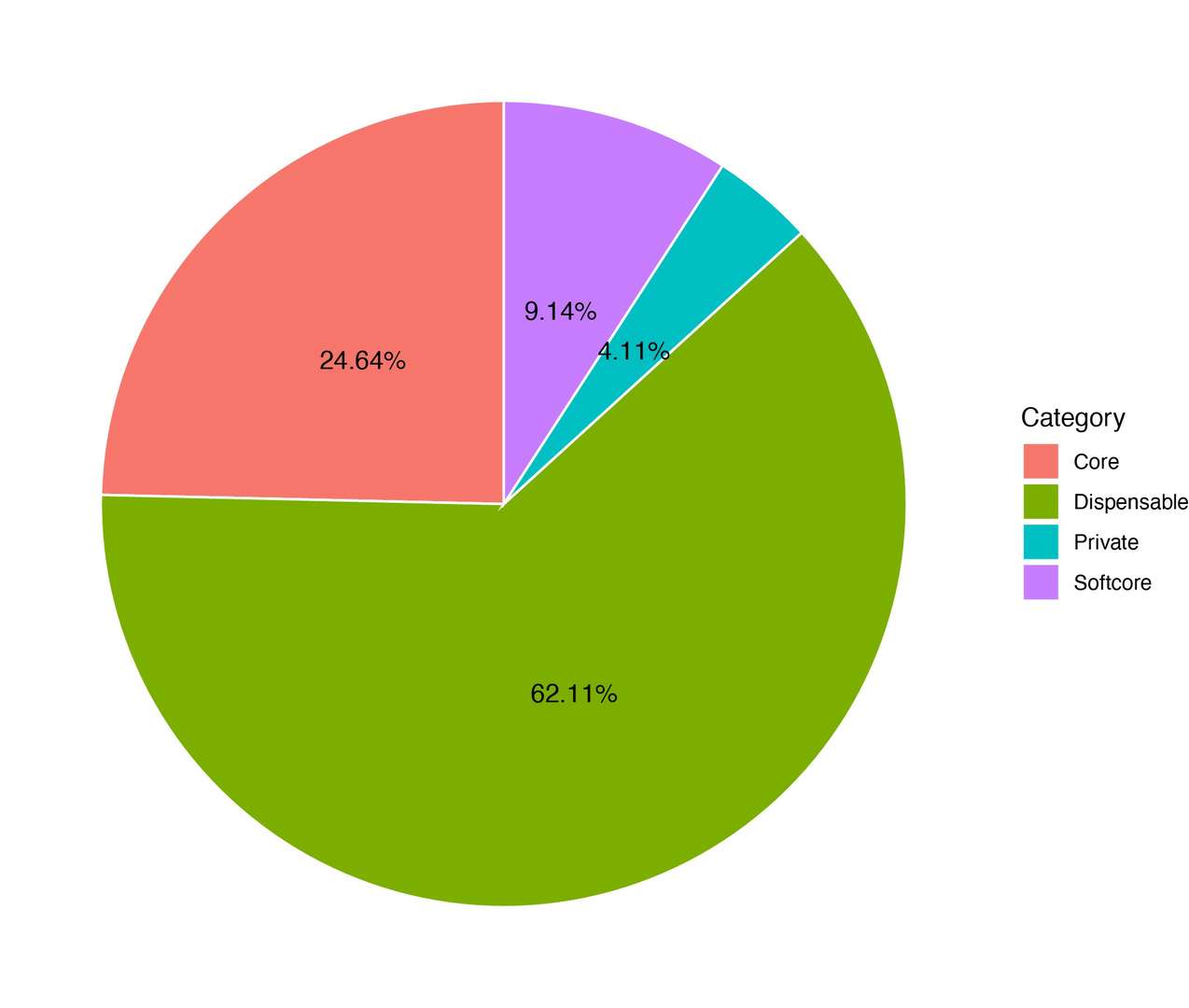 Figur2 . The proportion of genes in each category.
6.2 Frequency Histograms
Purpose: Display the distribution of gene presence frequencies, highlighting category thresholds.
ggplot(df_summary, aes(x = frequency, fill = Category)) +
 geom_histogram(binwidth = 0.05, alpha = 0.8) +
 scale_fill_manual(values = c("#F8766D", "#7CAE00", "#00BFC4", "#C77CFF")) +
 labs(x = "Presence Frequency", y = "Number of Genes",
 title = "Gene Frequency Distribution (Pan/Core Genes)") +
 theme_minimal() +
 geom_vline(xintercept = c(0.9, 1/n_samples), linetype = "dashed")
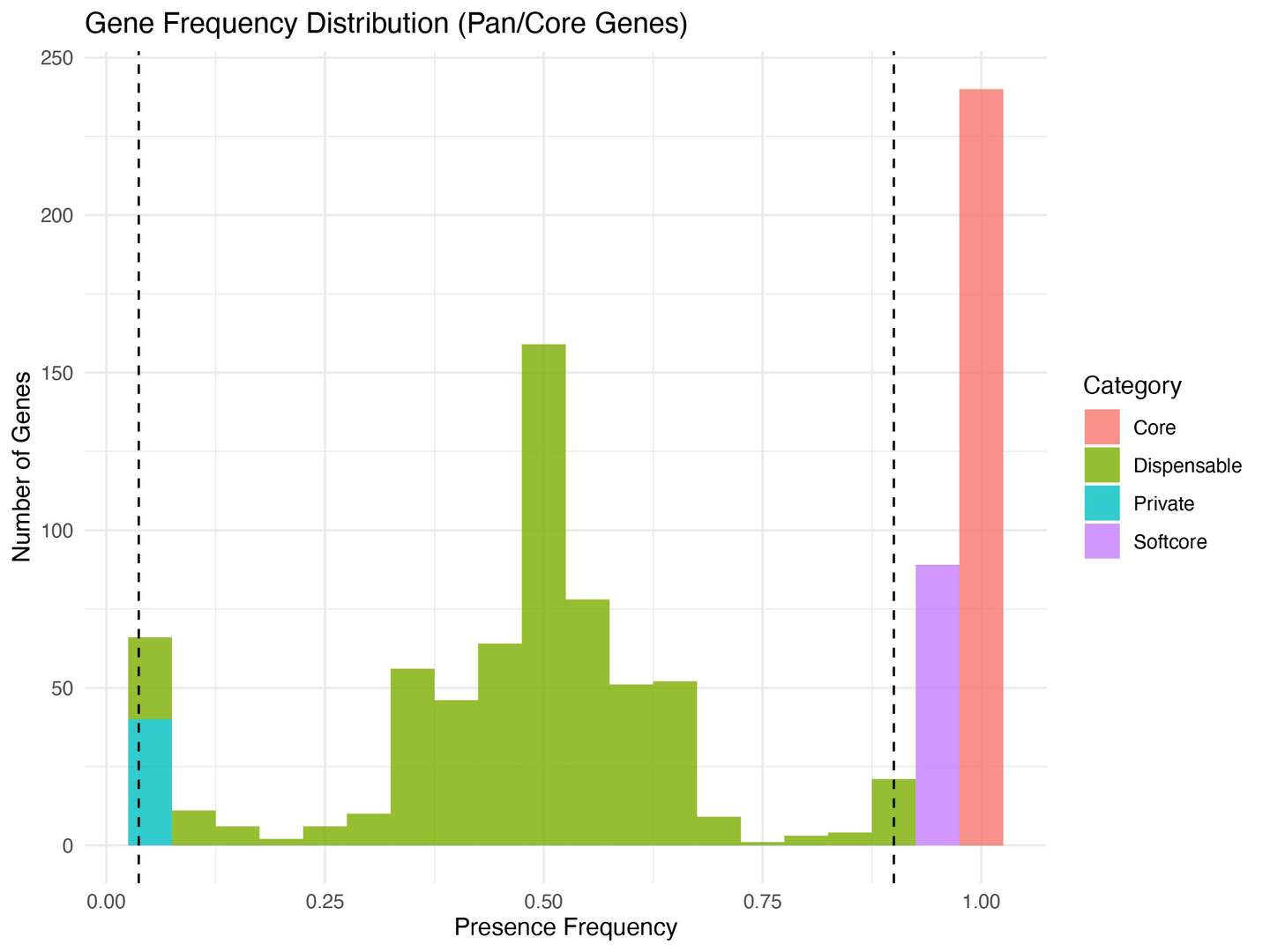 Figur3 . The distribution of gene presence frequencies.
6.3 Stacked Bar Charts
Purpose: Compare gene category composition across individual genomes or sample groups.
# Reshape matrix to long format and merge with gene category info
df_long <- df_combined %>%
 as.data.frame() %>%
 rownames_to_column("gene") %>%
 pivot_longer(-gene, names_to = "Sample", values_to = "Presence") %>%
 left_join(df_summary, by = "gene") %>%
 filter(Presence == 1)

# Calculate proportion of each category per sample
df_stack <- df_long %>%
 group_by(Sample, Category) %>%
 summarise(Count = n(), .groups = "drop") %>%
 group_by(Sample) %>%
 mutate(Proportion = Count / sum(Count))

ggplot(df_stack, aes(x = Sample, y = Proportion, fill = Category)) +
 geom_bar(stat = "identity", position = "fill") +
 ylab("Proportion of Genes") +
 theme_minimal() +
 theme(axis.text.x = element_text(angle = 90, hjust = 1))
Useful for population-level comparisons and revealing sample-specific enrichment patterns.
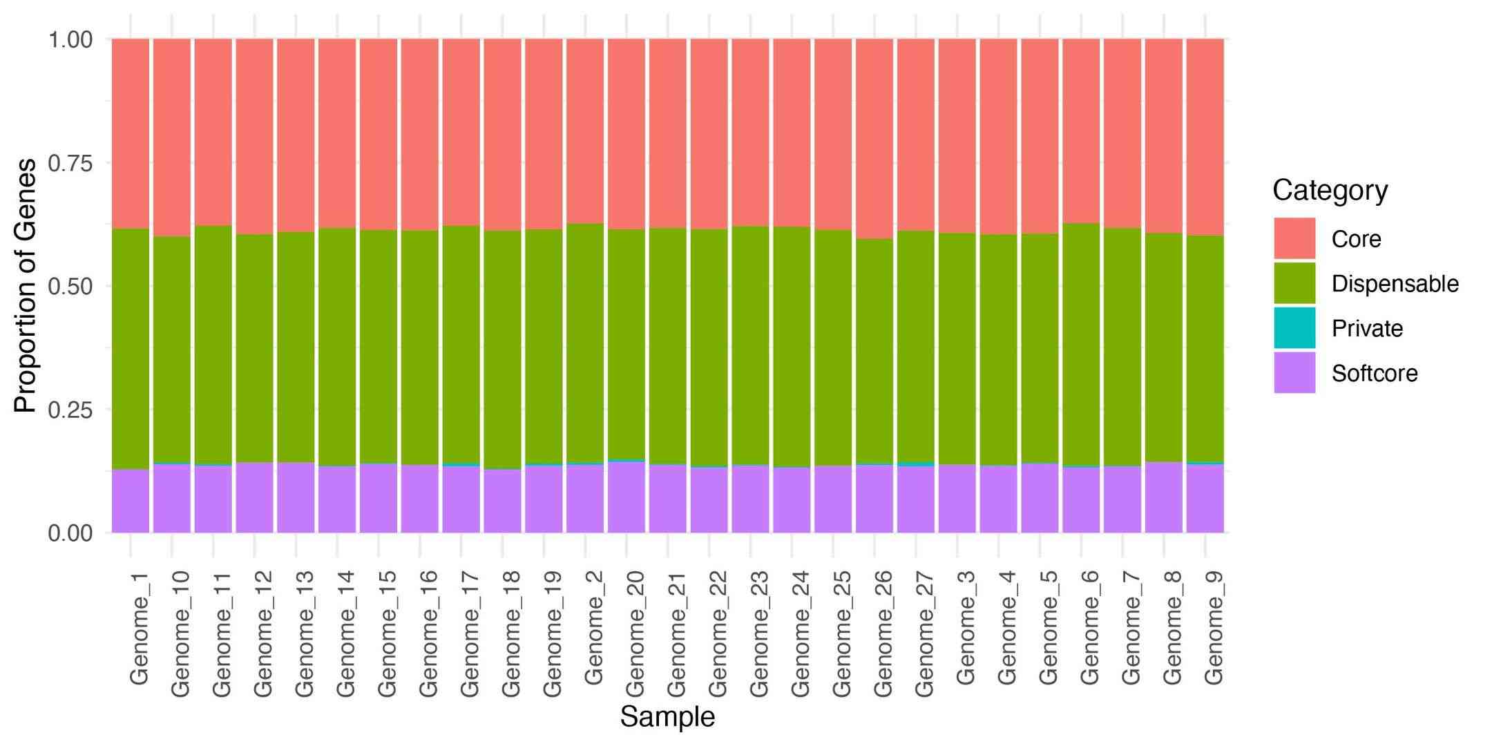 Figur4 . Gene category composition across individual genomes.
6.4 Heatmaps of Gene Presence/Absence
Purpose: Cluster genomes and genes to reveal structure and potential functional modules.
library(pheatmap)
row_order <- order(rowMeans(binary_matrix), decreasing = TRUE)
binary_matrix <- binary_matrix[row_order, ]
pheatmap(binary_matrix,
 color = c("#2166AC", "#B2182B"),
 show_rownames = FALSE,
 show_colnames = TRUE,
 cluster_rows = FALSE,
 cluster_cols = FALSE,
 breaks = seq(0, 1, length.out = 3),
 legend = TRUE,
 legend_breaks = c(0, 1),
 legend_labels = c("Absence", "Presence"),
 main = "Gene Presence/Absence in 27 Genomes",
 annotation_row = data.frame(Category=df_summary$Category, row.names=df_summary$gene),
 annotation_colors = list(Category = c(Core="#F8766D", Softcore="#7CAE00",
   Dispensable="#00BFC4", Private="#C77CFF")))
Clusters may correspond to subpopulations, ecotypes, or selective pressures.
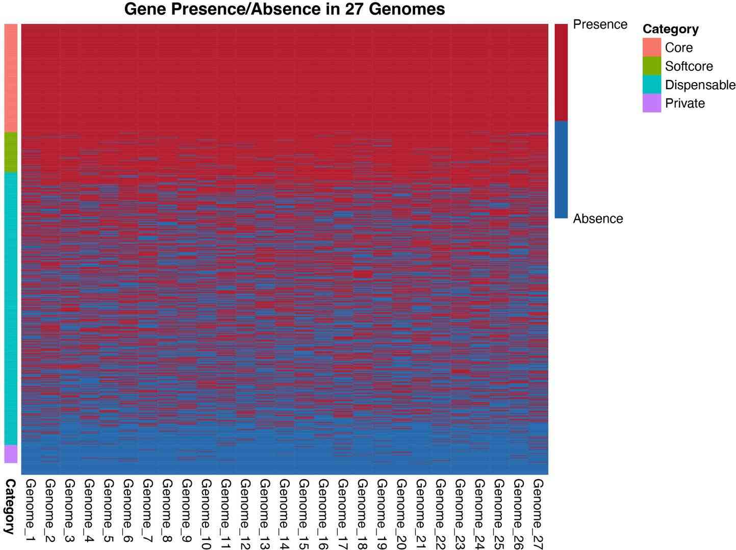 Figur5 . Presence and absence information of all gene families.
7. Conclusion
Pan-genome analysis provides a comprehensive framework for characterizing intra-species genomic variation. Classifying genes into core, softcore, dispensable, and private categories enables researchers to prioritize essential genes, identify adaptive features, and assess population diversity. By integrating robust pipelines like PSVCP for structural variation calling and tools such as OrthoFinder for gene family clustering, researchers can derive high-resolution presence/absence matrices essential for downstream analysis. Combined with quantitative profiling and intuitive visualization techniques-ranging from pie charts to hierarchical heatmaps-these strategies offer powerful insights into genome evolution, population structure, and functional diversity, thus paving the way for more informed genomic selection and association studies in both basic and applied research.
References:
- Li, X., Wang, Y., Cai, C. et al. Large-scale gene expression alterations introduced by structural variation drive morphotype diversification in Brassica oleracea. Nat Genet 56, 517–529 (2024). https://doi.org/10.1038/s41588-024-01655-4


