Metagenomic Sequencing Data: Step-by-Step Guide From Quality Check to Insights

Introduction

Metagenomic sequencing data analysis unlocks hidden stories about complex microbial ecosystems. By following a clear metagenomic analysis workflow, researchers can transform raw reads into actionable knowledge-discovering new species, tracking antibiotic-resistance genes, and mapping metabolic networks. This guide walks you through every essential checkpoint:

• Data-integrity checks to confirm file completeness
• Quality control and host-DNA removal for cleaner downstream results
• Assembly and binning strategies that build contigs and MAGs
• Gene prediction, abundance calculation, and annotation for functional insight
• Statistical testing and visualisation that reveal biological meaning

Whether you study human gut microbiomes or deep-sea sediments, the step-by-step tips below will strengthen your metagenomic sequencing data analysis from start to finish.

1 Data-Integrity Assessment

The preliminary validation phase comprises verification of file size, successful decompression, and absence of character corruption. Cryptographic hashing with md5sum is then applied to confirm byte-level fidelity of the sequencing archives.

2 Data Pre-processing

Metagenomic pipelines typically proceed via two principal trajectories. The first assembles short reads into contigs for downstream gene prediction and functional interrogation. The second constructs metagenome-assembled genomes (MAGs) through binning, followed by taxonomic profiling and differential functional-gene analysis (Figure 1).

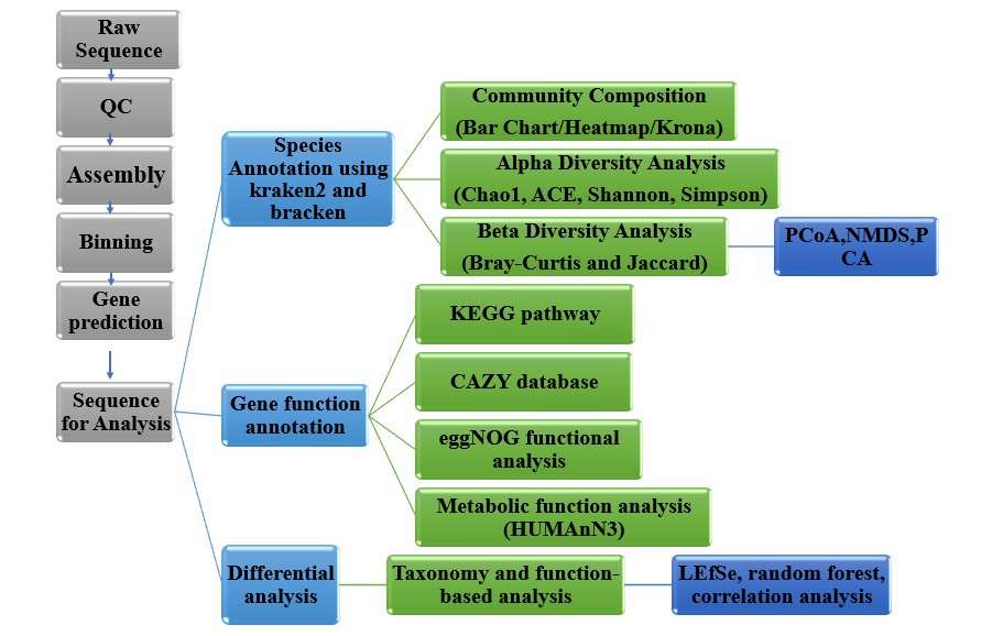Figure 1. Brief process of metagenomic analysis.

2.1 Quality Control

Raw Illumina reads (FASTQ) often contain adaptor sequences and low-quality bases. Read-quality visualisation is performed with FastQC (Andrews 2010), whereas Trimmomatic embedded in KneadData removes adaptors and trims substandard nucleotides (Bolger et al. 2014). Prior to processing, paired-end files are renamed with "_1" and "_2" suffixes to ensure software compatibility. MultiQC aggregates quality metrics across multiple samples into a unified report (Ewels et al. 2016). Libraries are generally accepted when ≥85 % of bases exhibit Phred scores ≥30 (Q30) and when GC content falls within the expected range.

2.2 Host Sequence Removal

Specimens originating from host-associated environments frequently harbour host DNA that diminishes microbial signal. Reference genomes obtained from Ensembl Genomes are indexed, and reads are aligned with Bowtie2, BWA, KneadData, or Kraken2 to remove host sequences (Langmead et al. 2009; Li and Durbin 2009; Wood et al. 2019). Benchmarking indicates that Kraken2 affords superior processing speed and reduced resource consumption (Gao et al. 2025) (Figure 2). A secondary FastQC evaluation confirms improvement. In a representative study, Bowtie2 alignment to the human reference genome (GRCh38) eliminated 98 % of host reads, increasing the detection sensitivity for Clostridioides difficile from 50 % to 90 % and markedly enhancing antimicrobial-resistance gene profiling (Kok et al. 2022).

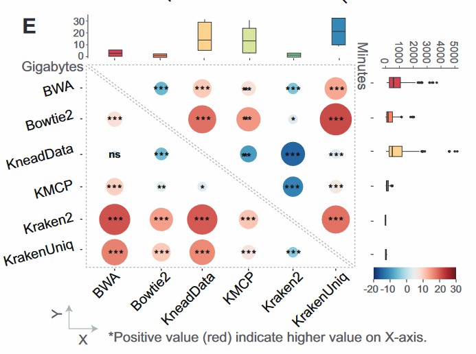Figure 2. Memory usage (top-right diagonal) and execution time (bottom-left diagonal) among different software (Gao et al. 2025).

3 Sequence Assembly and Binning

3.1 De novo Assembly

Short-read libraries are converted to contiguous sequences (contigs) with MEGAHIT (Li et al., 2015) or metaSPAdes (Bankevich et al., 2012). K-mer length, typically an odd integer, exerts a determinant effect on assembly efficiency and accuracy; optimal values may be inferred with KmerGenie (Chikhi and Medvedev, 2014). metaSPAdes produces contigs of superior fidelity albeit at greater computational cost, rendering it suitable for single-sample projects, whereas MEGAHIT affords rapid co-assembly across multiple samples. For a 252 Gb soil dataset, GPU-accelerated MEGAHIT concluded assembly within 44.1 h, tripling N50 and mean contig length relative to conventional methods and elevating the read-mapping rate to 55.8 %-a four-fold enhancement (Li et al., 2015). Increased N50 values reflect improved assembly continuity.

3.2 Binning and Genome Reconstruction

Assembled contigs are clustered into metagenome-assembled genomes (MAGs) via MetaBAT 2 (Kang et al., 2019) or related algorithms. Outputs from MaxBin 2, MetaBAT 2, and CONCOCT are routinely integrated with the MetaWRAP workflow (Uritskiy et al., 2018). The bin_refinement module reassembles draft genomes while enforcing user-defined completeness and contamination thresholds; quant_bins subsequently maps sample reads to each bin to quantify relative abundance. Application of this protocol to Cambodian fermented soybean (Sieng) microbiota yielded six high-quality MAGs (Tamang et al., 2023), whereas a separate investigation dereplicated 126 MAGs into 58 non-redundant genomic datasets (Banchi et al., 2023) (Figure 3).

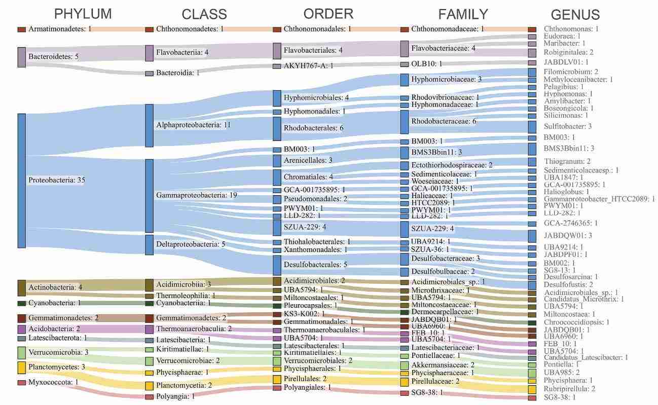Figure 3. A study constructed 58 non-redundant genomic datasets from 126 metagenomic assembly genomes (MAGs). (Banchi et al. 2023)

4 Gene Prediction and Redundancy Elimination

Open reading frames and non-coding RNAs are annotated with Prokka (parameter --metagenome), which embeds Prodigal and Infernal to derive corresponding protein sequences (Seemann 2014). Resultant fasta files may be further curated with SeqKit. Signal peptides are inferred with SignalP 6.0, whereas transmembrane helices-and, by extension, secreted proteins-are detected with TMHMM.

To mitigate inflation caused by highly similar sequences, predicted proteins are clustered with CD-HIT or MMseqs2, thereby generating a non-redundant gene catalogue (Unigene set) suitable for quantitative and functional analyses (Fu et al. 2012; Steinegger and Söding 2017). Similarity thresholds are adjusted in accordance with project objectives. This strategy enabled the recovery and functional annotation of metagenome-derived genes from Venice Lagoon sediments (Figure 4; Marine Bioscience and Technology study).

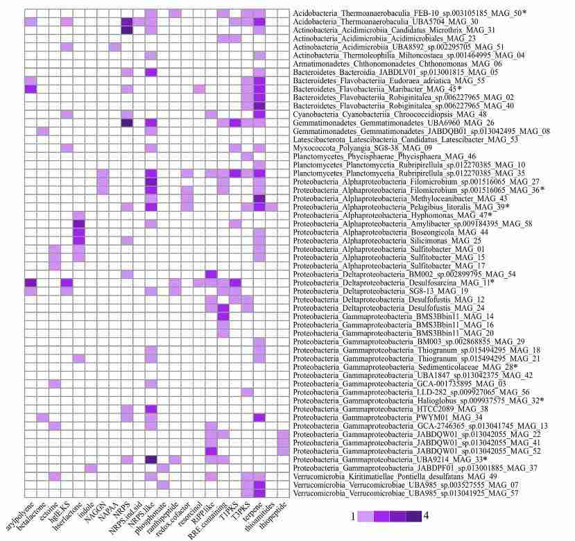Figure 4. Heatmap of the biosynthetic gene clusters (BGCs) detected in the MAG dataset (Banchi et al. 2023).

5 Quantification of Gene Abundance

Gene-abundance profiling provides relative or absolute estimates of specific loci within microbial consortia and, consequently, infers community metabolic capacity. Two widely adopted strategies are summarised below.

Gene-abundance profiling provides relative or absolute estimates of specific loci within microbial consortia and, consequently, infers community metabolic capacity. Two widely adopted strategies are summarised below.

• Read-mapping strategy. Sequencing reads are aligned to a non-redundant gene catalogue (Unigenes) with BWA or Bowtie 2. Per-gene coverage is subsequently calculated with CoverM and normalised as transcripts per million (TPM), reads per kilobase per million (RPKM), or unnormalised counts (Mortazavi et al., 2008; Corchete et al., 2020). TPM affords robust cross-sample comparison, whereas RPKM remains preferable for single-end libraries.
• k-mer-based strategy. Alignment-free estimation is performed with Salmon, which derives abundance directly from k-mer frequencies, thereby reducing computational overhead.

6 Taxonomic and Functional Annotation

6.1 Taxonomic Profiling

Taxonomic reconstruction elucidates community composition and facilitates the discovery of novel taxa. Three complementary algorithms are routinely employed:

• Kraken 2 classifies reads through k-mer hashing and achieves high sensitivity, particularly for low-abundance organisms, although an elevated false-positive rate has been reported.
• MetaPhlAn 4 exploits clade-specific marker genes to provide species-level precision, yet it may overlook taxa lacking canonical markers.
• GTDB-Tk identifies universal marker genes, generates multiple-sequence alignments, and performs phylogenomic placement, thereby offering refined classification of previously undescribed lineages (Chaumeil et al., 2020; Manghi et al., 2023).

In standard workflows, MetaPhlAn 4 supplies the core taxonomic profile; Kraken 2 augments detection of rare species; and GTDB-Tk resolves ambiguous or novel clades. Critical assignments are verified manually with BLAST searches. Community structure and phylogenetic relationships for the present study are illustrated in Figures 5 and 6.

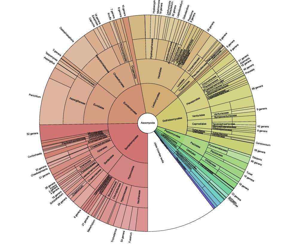Figure 5. Taxonomic profile of the Ascomycota component in the samples based on a Krona chart (Tedersoo et al. 2021).

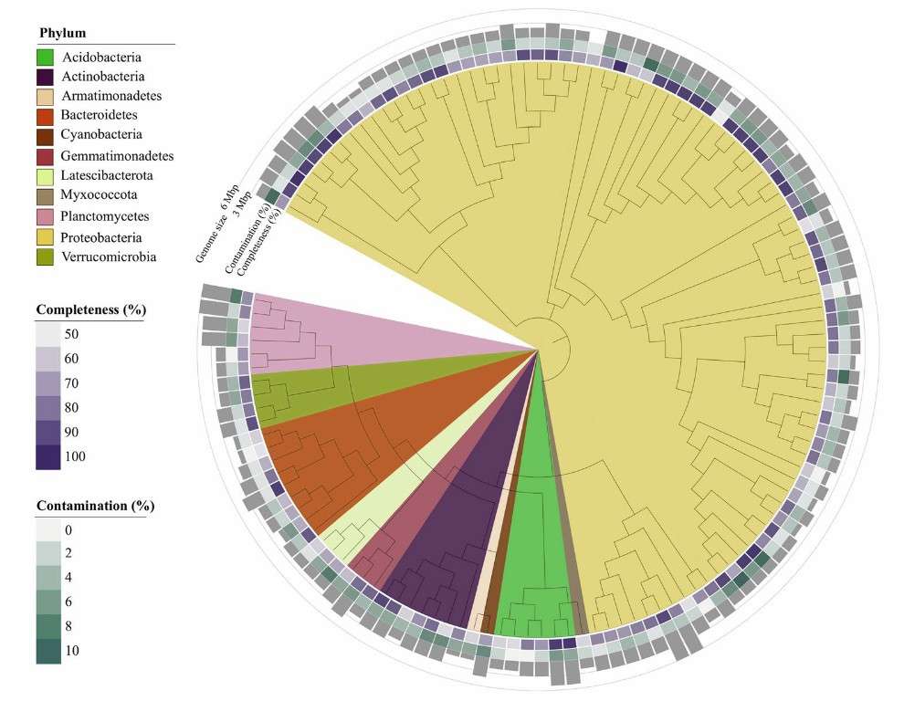Figure 6. Phylogenetic tree of MAGs reconstructed from Venice Lagoon sediment, based on a concatenated alignment of 43 conserved marker genes.(Banchi et al. 2023)

6.2 Functional Annotation

Initial functional prediction of metagenome-assembled genomes (MAGs) was conducted with Prokka, which integrates Prodigal and Infernal for open-reading-frame and RNA annotation. Orthologous groups were subsequently assigned with eggNOG-mapper against the eggNOG database (Huerta-Cepas et al.). Additional domain-specific analyses were undertaken in accordance with the study objectives: metabolic-pathway reconstruction with KofamKOALA; identification of carbohydrate-active enzymes via the CAZy repository; protease classification with the MEROPS database; antimicrobial-resistance gene detection using AMRFinderPlus; and prediction of community metabolic potential with HUMAnN 3 (Aramaki et al., 2020; Beghini et al., 2021).

The concatenated annotation pipeline enabled inference of carbon, nitrogen, and sulphur cycling genes, as well as biosynthetic gene clusters, within Venice Lagoon sediment MAGs (Figure 7; Banchi et al., 2023).

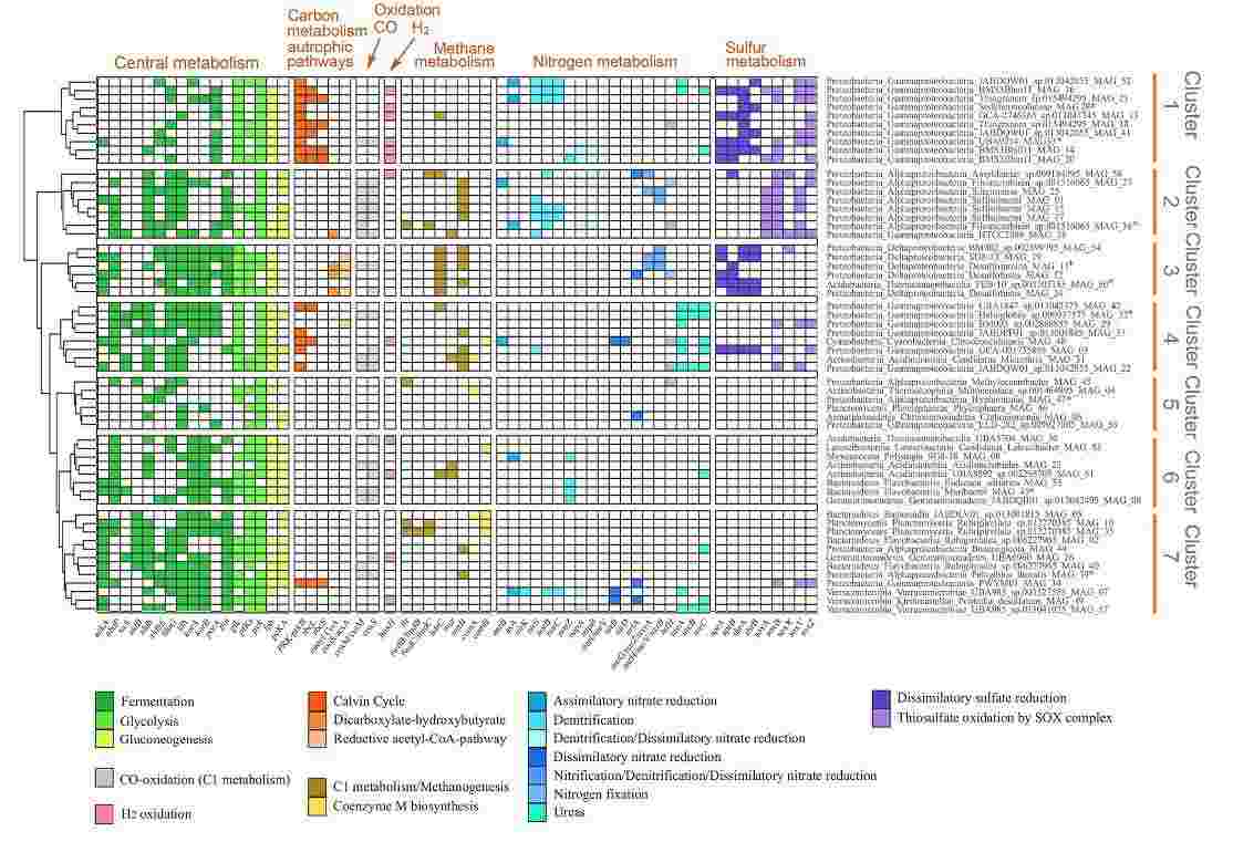Figure 7. Heatmap showing the metabolic potential of the MAGs based on the presence of key genes and metabolic pathways (Banchi et al. 2023).

7 Data Analysis and Visualisation

7.1 Statistical Evaluation of Gene Abundance

A gene-abundance matrix, normalised as transcripts per million (TPM) or raw read counts, was compiled for differential-expression analysis. Low-abundance features and batch effects were filtered prior to inference. Differential genes were identified with DESeq2 in R, applying an adjusted P < 0.05 and |log₂ fold-change| > 1. Additional feature selection employed linear discriminant analysis effect size (LEfSe; LDA score > 2) and random-forest classification. Where machine-learning models were implemented, candidate biomarkers exhibiting an area under the receiver-operating-characteristic curve (AUC) > 0.70 were deemed informative.

7.2 Complementary Analyses and Visualisation

Network association mapping, differential-gene plotting, and time-series evaluation were performed as required. Environmental drivers of community structure were interrogated with constrained ordination-canonical correspondence analysis (CCA) or redundancy analysis (RDA)-using the vegan package in R. Resultant ordinations were rendered with ggvegan and ggplot2, facilitating customised graphical output (Figure 8).

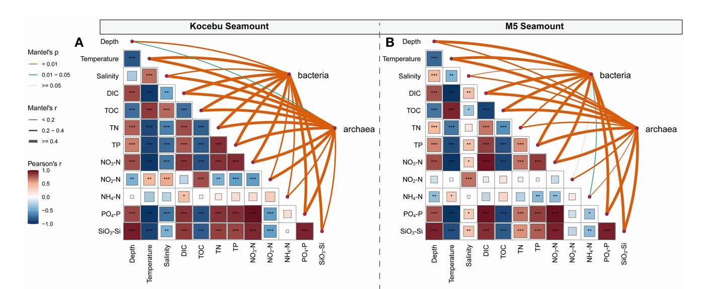Figure 8. Correlation analysis between environmental factors and microbial community composition (Liu et al. 2023).

Conclusion

Metagenomic studies succeed when every pipeline step-quality filtering, assembly, binning, annotation, and statistics-works in harmony. By:

• Verifying data integrity before analysis,
• Removing host contamination to sharpen microbial signals,
• Choosing assembly tools that fit dataset size and goals,
• Refining MAGs and non-redundant gene catalogues, and
• Linking taxonomy, function, and environment with rigorous statistics,

researchers gain a panoramic view of microbial diversity and function. Adopting these best-practice checkpoints will boost accuracy, cut processing time, and help translate sequencing reads into ecological or clinical insight. As tools evolve, regularly benchmarking new software against your existing workflow ensures your metagenomic sequencing tips stay future-proof and reproducible.

References:

1. Andrews, S. (2010). FastQC: A quality control tool for high throughput sequence data.
2. Aramaki T, Blanc-Mathieu R, Endo H, Ohkubo K, Kanehisa M, Goto S, Ogata H (2020) KofamKOALA: KEGG Ortholog assignment based on profile HMM and adaptive score threshold. Bioinformatics 36:2251-2252. https://doi.org/10.1093/bioinformatics/btz859
3. Banchi E, Corre E, Del Negro P, Celussi M, Malfatti F (2023) Genome-resolved metagenomics of Venice Lagoon surface sediment bacteria reveals high biosynthetic potential and metabolic plasticity as successful strategies in an impacted environment. Mar Life Sci Technol 6:126-142. https://doi.org/10.1007/s42995-023-00192-z
4. Bankevich A, Nurk S, Antipov D, Gurevich AA, Dvorkin M, Kulikov AS, Lesin VM, Nikolenko SI, Pham S, Prjibelski AD, Pyshkin AV, Sirotkin AV, Vyahhi N, Tesler G, Alekseyev MA, Pevzner PA (2012) SPAdes: A New Genome Assembly Algorithm and Its Applications to Single-Cell Sequencing. Journal of Computational Biology 19:455-477. https://doi.org/10.1089/cmb.2012.0021
5. Beghini F, McIver LJ, Blanco-Míguez A, Dubois L, Asnicar F, Maharjan S, Mailyan A, Manghi P, Scholz M, Thomas AM, Valles-Colomer M, Weingart G, Zhang Y, Zolfo M, Huttenhower C, Franzosa EA, Segata N (2021) Integrating taxonomic, functional, and strain-level profiling of diverse microbial communities with bioBakery 3. eLife 10:e65088. https://doi.org/10.7554/eLife.65088
6. Bolger AM, Lohse M, Usadel B (2014) Trimmomatic: a flexible trimmer for Illumina sequence data. Bioinformatics 30:2114-2120. https://doi.org/10.1093/bioinformatics/btu170
7. Chaumeil P-A, Mussig AJ, Hugenholtz P, Parks DH (2020) GTDB-Tk: a toolkit to classify genomes with the Genome Taxonomy Database. Bioinformatics 36:1925-1927. https://doi.org/10.1093/bioinformatics/btz848
8. Chikhi R, Medvedev P (2014) Informed and automated k -mer size selection for genome assembly. Bioinformatics 30:31-37. https://doi.org/10.1093/bioinformatics/btt310
9. Corchete LA, Rojas EA, Alonso-López D, De Las Rivas J, Gutiérrez NC, Burguillo FJ (2020) Systematic comparison and assessment of RNA-seq procedures for gene expression quantitative analysis. Sci Rep 10:19737. https://doi.org/10.1038/s41598-020-76881-x
10. Ewels P, Magnusson M, Lundin S, Käller M (2016) MultiQC: summarize analysis results for multiple tools and samples in a single report. Bioinformatics 32:3047-3048. https://doi.org/10.1093/bioinformatics/btw354
11. Fu L, Niu B, Zhu Z, Wu S, Li W (2012) CD-HIT: accelerated for clustering the next-generation sequencing data. Bioinformatics 28:3150-3152. https://doi.org/10.1093/bioinformatics/bts565
12. Gao Y, Luo H, Lyu H, Yang H, Yousuf S, Huang S, Liu Y-X (2025) Benchmarking short-read metagenomics tools for removing host contamination. GigaScience 14:giaf004. https://doi.org/10.1093/gigascience/giaf004
13. Huerta-Cepas J, Szklarczyk D, Heller D, Forslund SK, Cook H, Mende DR, Letunic I, Rattei T, Jensen LJ eggNOG 5.0: a hierarchical, functionally and phylogenetically annotated orthology resource based on 5090 organisms and 2502 viruses. https://doi.org/10.1093/nar/gky1085
14. Kang DD, Li F, Kirton E, Thomas A, Egan R, An H, Wang Z (2019) MetaBAT 2: an adaptive binning algorithm for robust and efficient genome reconstruction from metagenome assemblies. PeerJ 7:e7359. https://doi.org/10.7717/peerj.7359
15. Kok NA, Peker N, Schuele L, De Beer JL, Rossen JWA, Sinha B, Couto N (2022) Host DNA depletion can increase the sensitivity of Mycobacterium spp. detection through shotgun metagenomics in sputum. Front Microbiol 13:949328. https://doi.org/10.3389/fmicb.2022.949328
16. Langmead B, Trapnell C, Pop M, Salzberg SL (2009) Ultrafast and memory-efficient alignment of short DNA sequences to the human genome. Genome Biol 10:R25. https://doi.org/10.1186/gb-2009-10-3-r25
17. Li D, Liu C-M, Luo R, Sadakane K, Lam T-W (2015) MEGAHIT: an ultra-fast single-node solution for large and complex metagenomics assembly via succinct de Bruijn graph. Bioinformatics 31:1674-1676. https://doi.org/10.1093/bioinformatics/btv033
18. Li H, Durbin R (2009) Fast and accurate short read alignment with Burrows-Wheeler transform. Bioinformatics 25:1754-1760. https://doi.org/10.1093/bioinformatics/btp324
19. Liu N-H, Ma J, Lin S-Q, Xu K-D, Zhang Y-Z, Qin Q-L, Zhang X-Y (2023) Biogeographic distribution patterns of the bacterial and archaeal communities in two seamounts in the Pacific Ocean. Front Mar Sci 10:1160321. https://doi.org/10.3389/fmars.2023.1160321
20. Manghi P, Blanco-Míguez A, Manara S, NabiNejad A, Cumbo F, Beghini F, Armanini F, Golzato D, Huang KD, Thomas AM, Piccinno G, Punčochář M, Zolfo M, Lesker TR, Bredon M, Planchais J, Glodt J, Valles-Colomer M, Koren O, Pasolli E, Asnicar F, Strowig T, Sokol H, Segata N (2023) MetaPhlAn 4 profiling of unknown species-level genome bins improves the characterization of diet-associated microbiome changes in mice. Cell Reports 42:112464. https://doi.org/10.1016/j.celrep.2023.112464
21. Mortazavi A, Williams BA, McCue K, Schaeffer L, Wold B (2008) Mapping and quantifying mammalian transcriptomes by RNA-Seq. Nat Methods 5:621-628. https://doi.org/10.1038/nmeth.1226
22. Seemann T (2014) Prokka: rapid prokaryotic genome annotation. Bioinformatics 30:2068-2069. https://doi.org/10.1093/bioinformatics/btu153
23. Steinegger M, Söding J (2017) MMseqs2 enables sensitive protein sequence searching for the analysis of massive data sets. Nat Biotechnol 35:1026-1028. https://doi.org/10.1038/nbt.3988
24. Tamang JP, Kharnaior P, Das M, Ek S, Thapa N (2023) Metagenomics and metagenome-assembled genomes analysis of sieng, an ethnic fermented soybean food of Cambodia. Food Bioscience 56:103277. https://doi.org/10.1016/j.fbio.2023.103277
25. Tedersoo L, et al,. (2021) The Global Soil Mycobiome consortium dataset for boosting fungal diversity research. Fungal Diversity 111:573-588. https://doi.org/10.1007/s13225-021-00493-7
26. Uritskiy GV, DiRuggiero J, Taylor J (2018) MetaWRAP-a flexible pipeline for genome-resolved metagenomic data analysis. Microbiome 6:158. https://doi.org/10.1186/s40168-018-0541-1
27. Wood DE, Lu J, Langmead B (2019) Improved metagenomic analysis with Kraken 2. Genome Biol 20:257. https://doi.org/10.1186/s13059-019-1891-0