
 Sample Submission Guidelines
Pipeline and Tools for ChIP-Seq Analysis
What Is Chip-Seq Analysis?
Chromatin Immunoprecipitation sequencing (ChIP-seq) analysis serves as an indispensable technique in epigenomic research. This method employs antibodies that target specific DNA binding proteins or histone modifications to identify regions of enrichment within the genome. Utilization of histone modifications in ChIP-seq analysis allows for a profound dissection of epigenetic features and their biological functionalities. With advancements in Next Generation Sequencing (NGS) technologies and computational analyses, our understanding of the epigenomic landscape has substantially grown, informing us how it can contribute to cellular identity, development, lineage specification, and the etiology of a broad spectrum of conditions including cancer and other diseases.
Services you may interested in
Advantages of ChIP-Seq
- The ChIP-seq technology possesses the capacity to delineate at the nucleotide level, offering exquisitely detailed chromatin binding site information across entire genomes, thus shedding light on the intricacies of protein-DNA interactions. This empowers us to pinpoint with higher accuracy protein binding sites, such as those for transcription factors and histone modification enzymes.
- Contrary to ChIP-chip, there is an absence of noise generated from DNA fragment hybridization, where GC content, fragment length, concentration, and structural variances could meddle with hybridization.
- ChIP-seq enables genome-wide scanning, extending beyond the local area analysis. This broader scope allows a comprehensive understanding of the binding patterns of a certain protein at the genomic level, encompassing target gene identification and regulation.
- Quantitative chromatin binding signals offered by ChIP-seq data mirror the abundance and binding intensity of proteins in different genomic regions. This quantitative analysis facilitates comparison of chromatin binding patterns under varied conditions, and enables the identification of differential binding sites.
- The high-throughput sequencing characteristic of ChIP-seq allows the concurrent processing of a large number of samples and data, improving experimental efficiency. Furthermore, its high sensitivity enables detection of low-abundance protein binding sites, uncovering potential critical regulatory regions.
- ChIP-seq technology, independent of prior assumptions or primer design, exhibits minimal experimental bias and systematic error, leading to data that are more objective and reliable.
- ChIP-seq data can also be integrated with other omics data (such as RNA-seq, ATAC-seq, etc.) for comprehensive analysis to fully understand the complexities of gene expression regulatory networks. This integrative analysis contributes to elucidating the multilevel interactions between chromatin structure and gene regulation.
The Challenges of Chip-Seq
ChIP-seq is a powerful method to identify genome-wide DNA binding sites for a protein of interest. Mapping the chromosomal locations of transcription factors (TFs), nucleosomes, histone modifications, chromatin remodeling enzymes, chaperones, and polymerases is one of the key tasks of modern biology. To this end, ChIP-seq is the standard methodology (Bailey et al., 2013). Multiple challenges presented in ChIP-seq are not only in sample preparation and sequencing but also in computational analysis.
Unlike other types of massively parallel sequencing data, the ChIP-seq data have several characteristics:
- Histone modifications cover broader regions of DNA than TFs.
- Reads are trimmed to within a smaller number of bases.
- Fragments are quite large relative to binding sites of TFs.
- Measurements of histone modification often undulate following well-positioned nucleosomes.
To extract meaningful data from the raw sequence reads, the ChIP-seq data analysis should:
- Identify genomic regions - 'peaks' - where TF binds or histones are modified.
- Quantify and compare levels of binding or histone modification between samples.
- Characterize the relationships among chromatin state and gene expression or splicing.
Chip-Seq Bioinformatics Analysis Workflow
Bioinformatics analysis workflow for ChIP-seq data and the considerations for each step is illustrated in Figure 1 (Nakato and Shirahige, 2017). The procedure of sample preparation, sequencing and mapping (Figure 1A) is common in both experiments with single or a few samples (Figure 1B) and experiments with many samples (Figure 1C). Initially, sequencing reads of ChIP-seq are analyzed to assess the quality of the reads. After quality metrics, reads are mapped to the reference genome. Compared with input reads, genomic regions that are significantly enriched for ChIP reads are detected as peaks. Other genomic regions are regarded as non-specific background. Read densities can be visualized along the genome. Adjusting peak-calling strategy and parameters to each sample's property is possible in sample-scale analysis (Figure 1B). But one-by-one adjusting is difficult for large-scale analysis (Figure 1C), in which objective quality metrics for multilateral quantitative assessment is necessary to filter poor-quality data automatically. The called peaks represent candidates of histone modification and targeted protein or DNA-binding sites, which can be used to identify associated functional annotations, such as binding motifs.
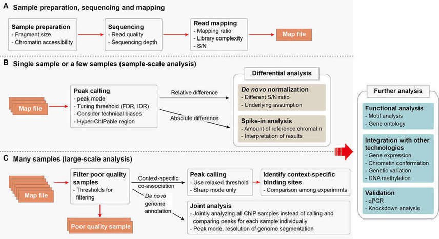 Figure 1. ChIP-seq analysis workflow. Adapted from (Nakato and Shirahige, 2017)
When conducting ChIP-Seq (Chromatin Immunoprecipitation Sequencing) data analysis, the processes generally observed are: handling of raw data, quality control analysis, mapping of reads, evaluation of read alignment quality, peak calling, annotation and analysis, among other primary steps.
Quality Control: The aim of the Quality Control (QC) step is to assess the substantive quality of high-throughput data produced from the sequencing. This includes inspecting the quality of raw sequencing data such as the length distribution of sequencing reads and the sequencing error rate. The most frequently used tool for such analysis is FastQC. Furthermore, should any sequences of low quality be identified, they can be discarded in subsequent trimming phases.
Read Mapping: The purpose of read mapping is to align trimmed sequencing reads with the reference genome. This aims to determine the precise genomic position of each read. Mapping tools such as Bowtie, Bowtie2, or BWA are typically employed for sequencing read mapping, with inputs being in FASTQ or CSFSATQ formats. Both Bowtie2 and BWA take into account indels (insertions and deletions) via gap alignment, making them suitable for long and/or paired-end reads.
Peak Calling: The step of peak identification concentrates on recognizing the areas of rich protein-DNA interaction throughout the genome. MACS2 is a commonly utilized tool in the analysis of ChIP-Seq data, highly functional in distinguishing enhanced areas within ChIP-Seq data, owing to its incorporation of genomic information and statistical models. However, the recent development of several peak calling tools adds to the repertoire of methods available. For instance, SICER is another application designed to identify enriched regions in ChIP-Seq data. By considering not only the prominence of the peaks but also their spatial distribution pattern, SICER may offer more acceptable outcomes compared to MACS2 under certain circumstances. Certain articles have suggested that utilizing distinct input DNA libraries as background controls can significantly impact peak detection. Generally, when employing an INPUT-seq library with greater sequencing depth for normalization, a greater number of peaks are identified as statistically significant, despite variations in the magnitude of disparities among different ChIP datasets.
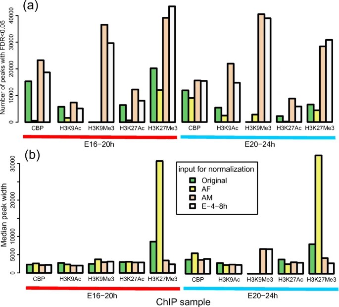 Figure 2. Effect of normalization with different INPUT-seq on ChIP-seq peak calling. (Ho et al., 2011)
Peak Annotation: Functional annotation of the identified enriched regions is performed, including functional classification of target genes, regulatory elements, etc. Tools predominantly used for this purpose include ChIPseeker and Homer.
Differential Analysis: Different conditions of ChIP-Seq data are compared to identify differences in enriched regions, in order to identify transcription factor target genes or changes in chromatin structure. Major tools used include DESeq2, edgeR, and so on.
Gene Set Enrichment Analysis: Tools such as GOseq and ChIP-Enrich are used to analyze the association between enriched regions and specific gene sets for functional annotation and biological interpretation.
Result Interpretation and Visualization: The biological interpretation of differential analysis results and enriched regions is carried out, checking the consistency with research hypotheses. Lastly, using tools such as IGV (Integrative Genomics Viewer), R packages (ggplot2, heatmap, etc.), the results from ChIP-Seq data are visualized, showcasing enriched regions, gene annotation and differential analysis results.
Chip-Seq Data Analysis Tools
There has been a large effort to improve analytical tools that are used in analysis of ChIP-seq data, and each step has led to the development of specialized software tools. A subset of software tools available for mapping and peak calling are briefly listed in Table 1 (Furey, 2012).
Table 1. A subset of software tools available for mapping and peak calling in the analysis of ChIP-seq data.
| Tool | Notes | Web address |
| Short-read aligners | ||
| BWA (Burrows-Wheeler Aligner) | Fast and efficient; based on the Burrows-Wheeler transform | http://bio-bwa.sourceforge.net |
| Bowtie | Similar to BWA, part of suite of tools that includes TopHat and CuffLinks for RNA-seq processing | http://bowtie-bio.sourceforge.net |
| GSNAP (Genomic Short-read Nucleotide Alignment Program) | Considers a set of variant allele inputs to better align to heterozygous sites | http://research-pub.gene.com/gmap |
| Wikipedia list of aligners | A comprehensive list of available short-read aligners, with descriptions and links to download the software | http://en.wikipedia.org/wiki/List_of_ sequence_alignment_software#Short- Read_Sequence_Alignment |
| Peak callers | ||
| MACS (Model-based Analysis for ChIP-seq) | Fits data to a dynamic Poisson distribution; works with and without control data | http://liulab.dfci.harvard.edu/MACS |
| PeakSeq | Takes into account differences in mappability of genomic regions; enrichment based on FDR (false-discovery rate) calculation | http://info.gersteinlab.org/PeakSeq |
| ZINBA (Zero-Inflated Negative Binomial Algorithm) | Can incorporate multiple genomic factors, such as mappability and GC content; can work with point-source and broad-source peak data | http://code.google.com/p/zinba |
Besides detection of enriched or bound regions in ChIP-seq data analysis, an important question is to determine differences between conditions. Owing to the complexity of ChIP-seq data in terms of noisiness and variability, the question is particularly challenging for ChIP-seq. Many different computational tools have been developed and published in recent years for differential ChIP-seq analysis. These tools show important differences in their algorithmic setups, in the number and size of detected differential regions (DR), and in the range of applicability. Description of 14 different tools for differential ChIP-seq data analysis is listed in Table 2 (Steinhauser et al., 2016).
Table 2. Description of different tools for differential ChIP-seq data analysis.
| Tool | Language | Peak Calling | Web address |
| SICER | Bash/Python | Window based approach, merging of eligible clusters in proximity closer than the defined gap size | https://home.gwu.edu/~wpeng/ Software.htm |
| MACS2 | Python | Not required | https://github.com/taoliu/MACS/ |
| ODIN | Python | Not required | http://costalab.org/wp/ odin |
| RSEG | C++ | Not required | http://smithlabresearch.org/software /rseg/ |
| MAnorm | R | Requires peak calling e.g. with MACS | http://bcb.dfci.harvard.edu/~gcyuan /MAnorm/MAnorm.htm |
| HOMER | Perl & C++ | Window based approach Peak calling done by HOMER | http://homer.salk.edu/homer /index.html |
| QChIPat | R, Perl & C++ | Peak calling possible with BELT, MACS, SISSRs or FindPeaks | http://motif.bmi.ohio-state.edu/ QChIPat/ |
| diffReps | Perl | Sliding window approach | https://github.com/shenlab -sinai/diffreps |
| DBChip | R | Requires peak calling e.g. with MACS | http://pages.cs.wisc.edu/ ~kliang/DBChIP/ |
| ChIPComp | R | Requires peak calling e.g. with MACS | http://web1.sph.emory.edu/users /hwu30/software/ChIPComp.html |
| MultiGPS | Java | Expectation maximization learning | http://mahonylab.org/software /multigps/ |
| MMDiff | R | Requires peak calling e.g. with MACS | https://bioconductor.riken.jp/ packages/3.1/bioc/html/MMDiff.html |
| DiffBind | R | Requires peak calling e.g. with MACS | http://bioconductor.org/packages /release/bioc/html/DiffBind.html |
| PePr | Python | Window based approach | https://github.com/shawnzhangyx /PePr |
Decision tree indicating the proper choice of tool is illustrated in Figure 3. The choice of tool depends on several factors: shape of the signal (sharp peaks or broad ChIP enrichments), presence of replicates and presence of an external set of regions of interest. The tools indicated in black give good results using default settings, and the tools in gray would require more extensive fine-tuning of parameters to achieve optimal results.
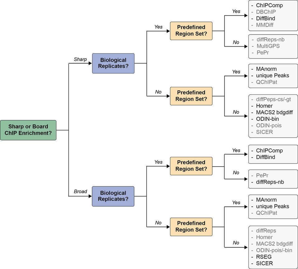 Figure 3. Decision tree indicating the proper choice of tool. Adapted from (Steinhauser et al., 2016).
Chip-Seq Data Analysis Technical Guidelines
Recent advances in sequencing technologies and analyses enable us to handle hundreds of ChIP samples simultaneously. But there are still some issues in analysis of ChIP-seq data, such as the false positive peaks, the multiple mapped reads and the poor overlap between peak-finding algorithm results. To obtain high-quality results from the computational analysis of ChIP-seq data, some technical aspects should be considered, which have been listed below (Bailey et al., 2013):
1) Sequencing Depth
Effective analysis of ChIP-seq data requires enough coverage by sequence reads (sequencing depth). The required sequencing depth mainly depends on the size of the genome and the number and size of the binding sites of the protein.
20 million reads may be adequate for mammalian TFs and chromatin modifications which are typically localized at specific, narrow sites, such as enhancer-associated histone marks (Landt et al., 2012).
Proteins with broader factors, including most histone marks, or more binding sites, such as RNA Pol II, will require up to 60 million reads for mammalian ChIP-seq (Chen et al., 2012).
Control samples should be sequenced significantly deeper than the ChIP ones.
2) Read Mapping and Quality Metrics
Before mapping to the reference genome, the reads should be filtered by applying a quality cutoff.
It is important to consider the percentage of uniquely mapped reads reported by the mapping tools.
3) Peak Calling
The analysis for ChIP-seq data is to predict the regions of the genome where the ChIPed protein is bound by finding regions with peaks.
A fine balance between sensitivity and specificity depends on choosing an appropriate peak-calling algorithm and normalization method based on the type of protein ChIPed.
4) Assessment of Reproducibility
To ensure the reproducibility of the experimental results, at least two biological replicates of each ChIP-seq experiment are recommended to be performed.
The reproducibility of both reads and identified peaks should be examined.
5) Differential Binding Analysis
Comparative ChIP-seq analysis of an increasing number of protein-bound regions across conditions or tissues is expected with the steady raise of NGS (next-generation sequencing) projects.
The direct calculation of differentially bound regions between treatment samples without controls is not recommended.
6) Peak Annotation
The aim of the annotation is to associate the ChIP-seq peaks with functionally relevant genomic regions, such as gene promoters, transcription start sites, intergenic regions, etc.
7) Motif Analysis
Motif analysis is useful for much more than just identifying the causal DNA-binding motif in TF ChIP-seq peaks.
When the motif of the ChIPed protein is already known, motif analysis provides validation of the success of the experiment.
Application of ChiP-Seq Data Analysis
ChIP-Seq is a technique widely applied in biological research. It delves into understanding protein-DNA interactions on chromatin, thereby elucidating gene regulatory mechanisms, epigenetics, and processes involved in disease progression and development. Epigenetic imbalances in disease versus healthy states might involve alterations in histone modifications and transcription factors. At this juncture, ChIP-Seq research has been employed to clarify the molecular pathologies of cancer and other diseases. It also has potential implications in deriving novel targets for diagnosing and treating diseases.
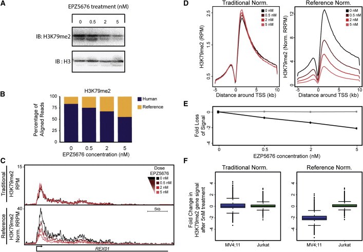 Figure 4. ChIP-Rx Reveals Epigenomic Alterations in Disease Cells that Respond to Drug Treatment. (Orlando et al., 2014)
ChIP-Seq has also proven to be valuable in providing insight into the role of transcription factors during disease progression. This tool enables the identification of transcription factor binding sites and regions of gene regulation such as histone modification sites, thereby plunging deeper into understanding the mechanisms governing gene regulation. ChIP-Seq analysis can determine the distribution patterns of histone modifications and DNA methylation across the genome, thereby revealing epigenetic regulatory networks and the impact of these modifications on gene expression and cellular functions. The results from ChIP-Seq are often employed in functional annotations to determine the biological processes and pathways that regulatory regions on the genome might participate in. This perspective clarifies the biological functionality of different genomic regions, promoting our understanding of intricate cellular dynamics.
As a technique extensively applied across diverse fields of biological research including developmental biology, oncology, and immunology, Chromatin Immunoprecipitation Sequencing (ChIP-Seq) offers vital insights into gene regulation and disease mechanisms. With the continual refinement and advancement of this technique, its role in unveiling intricate regulatory mechanisms within the genome and deciphering disease pathways will grow increasingly salient and pervasive.
Additional reading:
The Advantages and Workflow of ChIP-Seq
References:
- Bailey, T., Krajewski, P., Ladunga, I., et al. Practical guidelines for the comprehensive analysis of ChIP-seq data. PLoS computational biology, 2013, 9, e1003326.
- Chen, Y., Negre, N., Li, Q., et al. Systematic evaluation of factors influencing ChIP-seq fidelity. Nature methods, 2012, 9, 609-614.
- Furey, T.S. ChIP-seq and beyond: new and improved methodologies to detect and characterize protein-DNA interactions. Nature reviews Genetics, 2012, 13, 840-852.
- Landt, S.G., Marinov, G.K., Kundaje, A., et al. ChIP-seq guidelines and practices of the ENCODE and modENCODE consortia. Genome research, 2012, 22, 1813-1831.
- Machanick, P., and Bailey, T.L. MEME-ChIP: motif analysis of large DNA datasets. Bioinformatics, 2011, 27, 1696-1697.
- McLean, C.Y., Bristor, D., Hiller, M., et al. GREAT improves functional interpretation of cis-regulatory regions.Nature biotechnology, 2010, 28, 495-501.
- Nakato, R., and Shirahige, K. Recent advances in ChIP-seq analysis: from quality management to whole-genome annotation. Briefings in bioinformatics, 2017, 18, 279-290.
- Steinhauser, S., Kurzawa, N., Eils, R., and Herrmann, C. A comprehensive comparison of tools for differential ChIP-seq analysis. Briefings in bioinformatics, 2016, 17, 953-966.
- Thomas-Chollier, M., Herrmann, C., Defrance, M., Sand, O., Thieffry, D., and van Helden, J. RSAT peak-motifs: motif analysis in full-size ChIP-seq datasets. Nucleic acids research, 2012, 40, e31.
- Nakato R, Sakata T. Methods for ChIP-seq analysis: A practical workflow and advanced applications. Methods, 2021, 187: 44-53.
- Northrup D L, Zhao K. Application of ChIP-Seq and related techniques to the study of immune function. Immunity, 2011, 34(6): 830-842.
- Ho J W K, Bishop E, Karchenko P V, et al. ChIP-chip versus ChIP-seq: lessons for experimental design and data analysis. BMC genomics, 2011, 12: 1-12.
- Orlando D A, Chen M W, Brown V E, et al. Quantitative ChIP-Seq normalization reveals global modulation of the epigenome. Cell reports, 2014, 9(3): 1163-1170.


