ChIRP-MS Data Quality and Contaminant Control Guide
ChIRP‑MS can reveal RNA‑associated proteomes with remarkable breadth, but a long list is not a strong list. The credibility of a ChIRP-MS protein list hinges on five practical pillars: identification confidence (FDR), control-aware enrichment, background/contaminant review, replicate consistency, and a transparent path from discovery to a validation-ready shortlist. This article takes a firm stance—low FDR does not prove biological specificity—and turns that stance into an operational framework that teams can review, document, and apply consistently.
Key takeaways
- ChIRP‑MS data quality is defined by comparison structure and transparency, not by sheer protein count; the primary task is how to assess ChIRP‑MS data quality with controls, replicates, and documented filters.
- Low FDR establishes identification reliability, not mechanism; how to interpret FDR in ChIRP‑MS means separating statistical confidence from biological specificity in reporting and claims.
- To handle common contaminants in ChIRP‑MS, classify background sources (abundance, stickiness, indirect complex members, workflow carryover) and triage them before any pathway storytelling.
- A ChIRP‑MS validation ladder prioritizes candidates using reproducibility, control‑aware enrichment, biological plausibility, and feasibility—how to prioritize ChIRP‑MS candidates for validation requires an explicit, auditable ladder.
1. What Makes a ChIRP-MS List Credible
A credible ChIRP‑MS protein list is defined by reproducibility, control‑aware enrichment, and transparent filtering rather than by the number of detected proteins. Reviewers expect to see an audit trail that shows not just what survived, but why each protein survived.
1.1 What This Article Helps You Evaluate
This article clarifies what counts as a "credible list," what is "likely background," and which hits deserve to move into follow‑up validation. It provides a practical, reviewer‑oriented framework so teams can defend decisions in lab meetings, preprints, and peer review.
1.2 What to Check Before Interpreting Biology
Before diving into complexes, pathways, or mechanisms, check four things: (1) replicate consistency of enrichment; (2) the comparison structure against appropriate controls; (3) background flags for abundant and sticky proteins; and (4) the explicit filtering and prioritization logic. If any of these are unclear, detailed biological storytelling can wait.
1.3 What This Article Does Not Repeat
This guide does not re‑teach ChIRP‑MS basics or probe design. It focuses on result auditing and credibility judgments—what to look for in the data and how to justify the shortlist. For readers seeking practical service‑level context, see the internal overview of ChIRP-Seq & ChIRP-MS services.
2. Where Background Proteins Come From
Most background proteins in ChIRP‑MS come from abundant cellular components, sticky binders, indirect complexes, and workflow‑dependent carryover. Treating them as a single category leads to blunt filtering and lost signal. Classify first, then triage.
2.1 Abundant Proteins Are Not Automatically Meaningful
Highly abundant nuclear proteins, ribosomal proteins, cytoskeletal elements, and metabolic enzymes commonly appear in pull‑down MS datasets. Their presence alone does not imply a specific association with the target RNA. Baseline abundance must be contextualized against input controls and replicate patterns. Community practice and reviews of RNA‑interactome methods emphasize that abundance bias can masquerade as specificity when control design is weak or uneven.
2.2 Sticky Binders and Matrix Carryover Can Distort the List
Beads, surfaces, and sample handling can enrich nonspecific binders. These "sticky" proteins often recur across unrelated experiments. Bead‑only controls and cross‑checking with community contaminant resources help identify them, preventing a persistent false signal that would otherwise inflate the shortlist and mislead downstream narratives.
2.3 Indirect Complex Members Require Careful Interpretation
Many proteins co‑purify via complexes even if they never contact the RNA directly. Complex logic can be biologically informative—yet it must be interpreted as co‑enrichment, not direct binding. Without orthogonal evidence, an indirect complex member should not be promoted to "direct interactor."
2.4 Background Structure Changes Across Workflows
Hybridization conditions, crosslinking, lysis, wash stringency, and capture materials shape background structure. This guide stays at the result‑auditing level, but the implication is practical: background varies with method details, so contaminant logic should be visibly tied to the actual control structure and replicate behavior in your dataset.
 Figure 1. Background in ChIRP‑MS is heterogeneous—classify before filtering so triage is tailored rather than one‑size‑fits‑all.
3. How to Review Specificity Against Controls
Specificity in ChIRP‑MS is established by comparison structure, not by isolated enrichment values. Strong lists show how each control contributes to ruling out a source of noise.
3.1 What a Useful Control Comparison Should Answer
Controls must answer concrete questions: What is the baseline abundance? Which proteins adhere to beads or matrices regardless of the RNA? Which proteins bind without sequence specificity? Which enrichments are condition dependent? If the control suite cannot answer these, isolated fold changes will overstate specificity.
3.2 How Matched Controls Improve Confidence
Matched controls—input lysate, bead‑only, negative or scrambled probes, and condition‑matched samples—disentangle abundance effects, matrix stickiness, probe off‑targets, and biology‑dependent background. Their power is cumulative and complementary; no single control replaces the others.
3.3 Why One Strong Hit Is Not Enough
A single high‑scoring protein identified once without supportive controls and replicate consistency is a provisional observation. Isolated hits are usually treated cautiously unless the comparison structure shows that enrichment persists across relevant contrasts and replicates.
3.4 What Reviewers Usually Look for First
Reviewers first check whether the control architecture is appropriate for the question and whether enrichment remains consistent across the planned comparisons. They then examine how much of the list remains after removing proteins that match control‑dominated patterns.
 Figure 2. Different controls rule out different noise sources—none are interchangeable. Together they form the backbone for specificity judgments.
For readers comparing RNA‑protein capture strategies and their control logic, see the internal primer on RIP-Seq workflow, data analysis, and experimental design.
4. How to Read FDR Correctly
FDR helps control identification uncertainty, but it does not by itself prove biological specificity, direct binding, or mechanism. Treat FDR as the gatekeeper for reliable identifications, not as a shortcut to mechanistic claims.
4.1 What FDR Actually Helps With
At the spectrum/peptide/protein level, FDR (often via target‑decoy strategies) limits false identifications. Clear reporting of thresholds and formats is standard practice, and repositories expect explicit disclosure of search parameters and FDR choices. This ensures readers can trust that names on the list correspond to real identifications.
A reviewer-friendly default is to report FDR at the level(s) actually used for filtering (PSM, peptide, and/or protein) and to keep it explicit in tables (e.g., protein q-values). A common manuscript convention is a 1% threshold at the primary reporting level, but the key is consistency: the same level, threshold, and inference rules should be applied across target and controls and stated in the Methods or supplement.
4.2 What FDR Cannot Prove
Even at low FDR, a protein may be: (a) abundant background; (b) a sticky binder carried by beads or surfaces; or (c) an indirect complex member. FDR does not address any of these. Without control‑aware enrichment and replicate support, the leap from "identified confidently" to "specific interactor" is unjustified.
4.3 Why Statistical Confidence and Biological Specificity Are Different
Identification confidence is a statistical question: was this protein really detected? Biological specificity is a comparative and mechanistic question: is the enrichment target‑dependent and meaningful in context? These are distinct axes that must be reported and interpreted separately.
4.4 How to Explain FDR to Non-MS Readers
In one sentence: FDR addresses whether the identification is reliable; it does not tell whether the protein is a specific, mechanistically relevant partner of the target RNA. That second claim requires control comparisons, replicate consistency, and a credible rationale for biological fit.
 Figure 3. FDR governs identification confidence only. Low FDR ≠ direct binder.
For readers who want to connect identification reporting with general LC–MS/MS capabilities and deliverables, see the internal page on Epigenetic Modification Mass Spectrometry (LC–MS/MS) services.
5. How to Triage Contaminants Before Pathway Analysis
Contaminant review should happen before pathway storytelling; otherwise, compelling narratives may be built on noisy lists. Treat triage as a decision path that narrows the set to interpretable, defensible candidates.
5.1 A Practical Triage Order
A pragmatic sequence works well in practice: first, flag frequent background categories (abundant, sticky, and known contaminants); second, down‑rank proteins that appear equivalently in bead‑only or negative‑probe controls; third, require replicate presence of enrichment; only after these steps, move to potential complexes and pathways.
5.2 How to Separate Background From Contextual Proteins
Proteins that align with the cellular context but lack strong control/replicate support can be placed on a watch list rather than promoted to the main conclusions. This keeps the shortlist conservative while allowing follow‑up designs to probe context‑dependent roles.
5.3 Why Pathway Enrichment Can Amplify Noise
Enrichment analyses turn whatever structure exists in the input list into "significance." If the input retains abundance or stickiness artifacts, pathway outputs will echo that structure convincingly but spuriously. Pathway work should begin only after control‑driven and replicate‑driven cleaning.
5.4 What Should Stay Out of the Final Claims
Untriaged, full protein lists should not be used to write mechanism claims. Claims should be anchored to the shortlist that survives control comparison, contaminant review, and replicate consistency metrics.
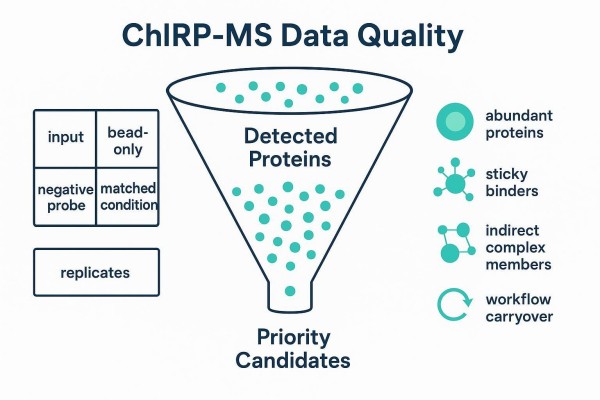
 Figure 4. The funnel from detection to a defensible shortlist relies on controls, contaminant flags, and replicate evidence.
For a broader overview of orthogonal and related approaches that help contextualize RNA‑centered interactomes, see the internal guide to molecular interaction mapping methods.
6. How to Build a Validation Ladder
A validation ladder turns a broad discovery list into a smaller, more defensible set of candidates for follow‑up. The aim is not maximal sensitivity at this stage, but auditability and feasibility.
6.1 Tier 1: Reproducible Enriched Proteins
Tier 1 retains proteins that are confidently identified, reproducibly enriched versus appropriate controls, and not frequent contaminants. Replicate presence and control‑aware fold change are the first gates.
One practical way to make "reproducible" auditable is to report a replicate presence fraction and predefine an inclusion rule. For example, some teams may retain candidates observed as enriched in at least 2 of 3 biological replicates (or 2 of 2 when only two replicates exist) and treat 1-of-N observations as provisional unless a clear technical rationale is documented. These example thresholds are illustrative only and should be adapted to study design, control architecture, and overall data quality.
6.2 Tier 2: Biologically Plausible Candidates
Tier 2 weighs cellular function, subcellular localization, known RNA biology, and complex membership. A protein that fits the biology but shows modest enrichment may remain in Tier 2 if it meets baseline replicate/control checks.
6.3 Tier 3: Mechanistically Actionable Proteins
Tier 3 highlights candidates that are best positioned for orthogonal validation and mechanistic assays. Criteria include clean control profiles, strong replicate evidence, and testable hypotheses. Cross‑method hints—for example, known RBP domains or prior evidence from orthogonal assays—can help prioritize.
6.4 What Makes a Good Shortlist
A good shortlist balances score, reproducibility, interpretability boundaries, and feasibility. It should be small enough to test, large enough to capture plausible diversity, and clearly annotated so each candidate's status is easy to audit.
Orthogonal assays often strengthen the case for specific interactions; readers can explore eCLIP-seq as one example of a complementary validation path.
Synthetic Example: From Discovery to Shortlist (Structure Only)
Below is a compact, synthetic example table that demonstrates how discovery hits can be triaged into a validation ladder. Values are illustrative placeholders to show structure and decision logic—not real findings.
| ProteinID | Gene | TargetAvgSpecCount | ControlAvgSpecCount | Log2FoldChange | qValue_FDR | ReplicatePresenceFraction | BackgroundFlag | ValidationTier | Notes |
|---|---|---|---|---|---|---|---|---|---|
| P12345 | RBP1 | 45 | 6 | 2.9 | 0.005 | 1.0 | None | Tier 3 | Strong enrichment vs bead‑only and negative probe; nuclear RBP domain |
| Q67890 | HSPX | 52 | 38 | 0.5 | 0.002 | 0.67 | Abundant | Watch | High abundance; modest FC; present in bead‑only; defer to watch list |
| A11111 | ACTN | 28 | 25 | 0.2 | 0.010 | 0.33 | Sticky | Remove | Cytoskeletal/sticky profile; recurrent in controls |
| B22222 | RBP2 | 18 | 3 | 2.6 | 0.020 | 1.0 | None | Tier 2 | Plausible RNA‑related function; consistent across replicates |
| C33333 | CMPLX | 12 | 2 | 2.6 | 0.030 | 0.67 | Indirect | Tier 1 | Co‑enriched complex member; needs orthogonal test |
Interpretation roadmap: (1) RBP1 passes all gates and is mechanistically actionable (Tier 3). (2) HSPX is abundant and partly present in controls—keep as a watch‑list item. (3) ACTN appears sticky and control‑dominated—remove. (4) RBP2 is reproducible, enriched, and plausible—Tier 2. (5) CMPLX is likely indirect—keep as Tier 1 with a note to test complex dependence.
7. How to Report ChIRP-MS Quality Clearly
Reviewer‑ready reporting makes the filtering logic, contaminant review, and candidate prioritization traceable. The goal is clarity: show where identification confidence ends and where specificity judgments begin.
7.1 What a Minimum Reporting Set Should Include
A concise minimum set typically covers: sample metadata (including probe set and major experimental conditions), control architecture and replicate counts, search parameters and FDR thresholds, explicit filtering logic, contaminant flags, and the derivation path for the shortlist. Repositories expect well‑formed identifiers and consistent metadata so peers can trace identification and enrichment claims.
A copy/paste-friendly deliverable template helps keep identification confidence separate from specificity judgments:
Candidate table (recommended columns): ProteinID (UniProt), Gene symbol, Protein-level q-value (FDR), Target vs bead-only log2FC, Target vs negative-probe log2FC, Replicate presence fraction, Background flag (Abundant/Sticky/Indirect/Carryover), Assigned tier (Tier 1–3 or Watch/Remove), Notes.
Minimum metadata to disclose (in Methods or supplement): probe set description (target and negative), crosslinking and major lysis/wash conditions (high level), control types included, biological replicate count, MS instrument and search software versions, database and variable modifications, FDR level(s) used for filtering, and the exact shortlist rules (thresholds and tie-breakers).
7.2 Which Tables and Figures Improve Interpretability
Tables that separate identification metrics (q‑values) from control‑aware enrichment (fold changes versus specific controls), replicate presence, and contaminant flags substantially improve interpretability. Figures that map controls to ruled‑out noise and show the funnel from detection to shortlist help readers audit judgment calls without combing through raw files.
7.3 Which Claims Should Be Softened
Co‑enrichment does not equal direct binding. Single‑experiment peaks without control and replicate support remain provisional. Phrases like "consistent with," "compatible with," or "suggests" are appropriate until orthogonal evidence clarifies mechanism.
7.4 How to Make the Shortlist Audit-Friendly
Each retained protein should carry a visible reason path: its control comparisons, replicate presence, background flags, assigned tier, and notes for orthogonal follow‑up. This allows others to reproduce the triage or debate thresholds constructively.
A provider‑style micro‑example (RUO): In practice, a deliverable may present a candidate table that lists identification q-values separately from control-aware enrichment (e.g., log2 fold change vs bead-only and negative probe), includes a replicate presence fraction, flags frequent contaminants, and labels a validation tier for each protein. This format keeps statistical confidence distinct from specificity, aligning with reviewer expectations for transparency. For analysis context, see the internal page on Epigenomic data analysis.
8. FAQs About ChIRP-MS Data Quality
8.1 How Do I Know Whether a ChIRP-MS Protein List Is Reliable?
Reliability shows up as patterns, not promises. Look for explicit FDR thresholds for identification, a control suite that addresses abundance, stickiness, probe off‑targets, and condition‑dependent background, and consistent enrichment across biological replicates. The final shortlist should show contaminant flags and a clear reason path from detection to prioritization.
8.2 Does a Lower FDR Mean a Protein Is a True Interactor?
Not necessarily. Lower FDR means the identification is statistically reliable. It does not prove target‑dependent binding or mechanism. Specificity depends on control‑aware enrichment and replicate behavior and should be presented as a separate dimension in the report.
8.3 What Proteins Are Commonly Considered Background in ChIRP-MS?
Abundant proteins (e.g., ribosomal, cytoskeletal, metabolic), sticky binders associated with beads or surfaces, and proteins co‑enriched through complexes are routinely flagged during review. Their status depends on control behavior and replicates; some may move to a watch list rather than be removed outright.
8.4 Should Pathway Analysis Be Done Before Contaminant Review?
It should not. Pathway analysis on an untriaged list will often convert background structure into "significant" pathways. Clean the list with controls, background flags, and replicate checks first; then interpret pathways from the refined set.
8.5 How Many Proteins Should Go Into Validation?
There is no fixed number. A defensible shortlist balances reproducibility, control‑aware enrichment, biological plausibility, and feasibility. Many programs favor a compact set that can be tested in a timely, interpretable fashion without diluting resources.
8.6 What Is the Difference Between Statistical Confidence and Biological Specificity?
Statistical confidence asks whether a protein was identified reliably (FDR space). Biological specificity asks whether the enrichment depends on the target RNA and is meaningful in context. Reports should keep these axes separate and label claims accordingly.
For broader method context that situates ChIRP alongside related RNA‑centric strategies, see the internal comparison of ChIRP-Seq, PIRCh-Seq, RIP-Seq, and CLIP/eCLIP comparison.
Pre‑Interpretation Pocket Checklist
- Controls address abundance, stickiness, probe off‑targets, and condition‑dependent background; replicates are present and appropriately matched.
- Identification thresholds and formats (including FDR) are explicit; enrichment is reported per control comparison, not as isolated numbers.
- Contaminant flags and watch‑list logic are documented; the shortlist includes reason paths and proposed orthogonal follow‑ups.
Closing Notes
ChIRP‑MS data quality is earned through comparison logic and transparency. Treat FDR as the first gate, not the final verdict. Classify background, require replicate evidence, and promote candidates onto a clearly labeled validation ladder. That way, the proteins carried forward into experiments are not just statistically credible—they are biologically defensible and audit‑friendly.
When teams need structured analysis deliverables, it helps to work with a provider that clearly separates identification confidence, control-aware enrichment, contaminant flags, and validation tiers in a transparent reporting format.
References and Further Reading (selected)
- HUPO‑PSI at Twenty Years (2023). Topology of the Human and Mouse m6A RNA Methylomes Revealed by m6A-seq.
- ProteomeXchange consortium update (2026, NAR). ProteomeXchange consortium update.
- Analytical Science Reviews (2024) on interaction MS. Summarizes contaminant-aware thinking.
- WIREs RNA review (2022). Context for RNA-centered capture strategies.